Zebrafish melanoma

You can download them from STMiner-test-data. You can also download the raw dataset from GEO.

Import package

from STMiner.SPFinder import SPFinder

Load data

file_path = 'Path/to/your/h5ad/file'
sp = SPFinder()
sp.read_h5ad(file=file_path, bin_size=1)

The parameter bin_size specifies the size of merged cells (spots). If not specified, no merging is performed. If set to 50, 50x50 cells/spots will be merged into a single cell/spot. Due to low sequencing depth in some datasets, cells/spots are often merged during analysis (e.g., stereo-seq). However, 10x data typically does not require merging.
The ST datasets was storaged in .adata object of sp, you can use sp.adata to check them:

sp.adata

Besides, sp Obj has many useful attributes which can be used for visualization or integrated into other pipelines (such as scanpy). See API for more details.

Find SVG

sp.get_genes_csr_array(min_cells=200, log1p=False)
sp.spatial_high_variable_genes(thread=6)

The parameter min_cells was used to filter genes that are too sparse to generate a reliable spatial distribution.
The parameter log1p was used to avoid extreme values affecting the results. For most open-source h5ad files, log1p has already been executed, so the default value here is False.
You can perform STMiner in your interested gene sets. Use parameter gene_list to input the gene list to STMiner. Then, STMiner will only calculate the given gene set of the dataset.
You can see output while computing as follows:

Parsing distance array...: 100%|██████████| 10762/10762 [01:12<00:00, 149.11it/s]
Computing ot distances...:  10%|▉         | 1069/10762 [03:04<31:11,  6.12it/s]  

You can check the spatial varitation of each gene by:

sp.global_distance

Gene	Distance	z-score
myha	1.35E+08	2.771493
vmhcl	1.01E+08	2.470881
zgc:101560	9.95E+07	2.458787
pvalb1	9.82E+07	2.445257
myhz2	9.75E+07	2.437787
...	...	...
rps17	2.61E+05	-3.63207
rpl13	2.48E+05	-3.68506
rpl32	2.43E+05	-3.70327
rsl24d1	2.27E+05	-3.7757
rpl22	1.83E+05	-3.99332

Fit GMM

sp.fit_pattern(n_comp=20, gene_list=list(sp.global_distance[:2000]['Gene']))

You can see output while computing as follows:

Fitting GMM...:  10%|▉         | 190/2000 [00:42<04:36,  6.54it/s] 

n_comp： Number of components for each GMM model
gene_list: Gene list to fit GMM model

Build distance array

sp.build_distance_array()

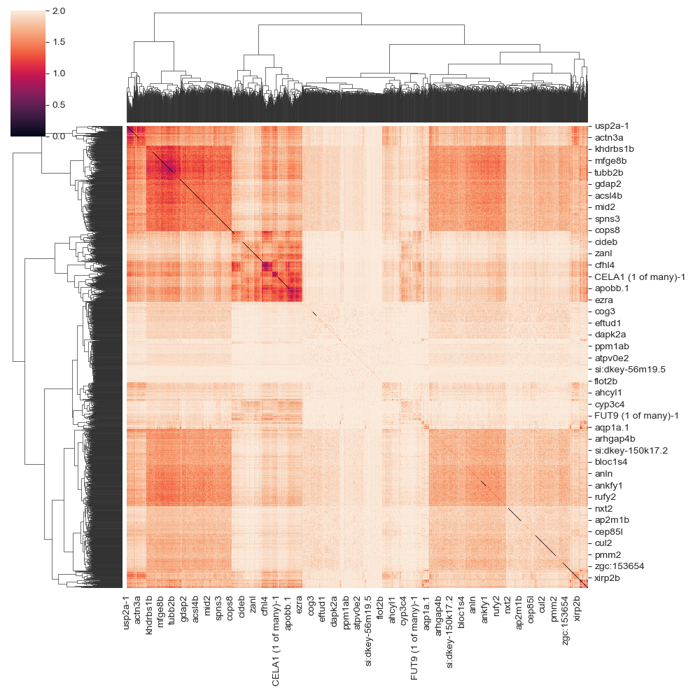
This step calculates the distance between genes’ spatial distributions. You can visualize the distance array by:

import seaborn as sns
sns.clustermap(sp.genes_distance_array)

build distance matrix & clustering

sp.cluster(n_clusters=6)

n_clusters: Number of cluster

Result & Visualization

The result are stored in genes_labels:

spf.genes_labels

The output looks like the following:

	gene_id	labels
0	Cldn5	2
1	Fyco1	2
2	Pmepa1	2
3	Arhgap5	0
4	Apc	5
..	...	...
95	Cyp2a5	0
96	X5730403I07Rik	0
97	Ltbp2	2
98	Rbp4	4
99	Hist1h1e	4

To visualize the patterns by heatmap:

sp.get_pattern_array()
sp.plot.plot_pattern(heatmap=False,
                     s=5,
                     rotate=True,
                     reverse_y=True,
                     reverse_x=True,
                     vmax=95,
                     cmap='Spectral_r',
                     output_path='./')

heatmap: If True, plot a heatmap. If False, plot a scatterplot. False is the default.
s: Spot size
rotate\reverse_y\reverse_x: Adjust the axis of plot.
cmap: cmap of plot
vmax: The percentage of the highest value of plots. Avoid the effect of large values for visualization.
output_path: If set, save the figure to path To visualize the genes by labels:

sp.plot.plot_genes(label=0, n_gene=8, s=5, reverse_y=True, reverse_x=True)

n_gene: Number of genes to visualize

To visualize the specific gene (such as BRAFhuman):

hcc2l.plot.plot_gene('BRAFhuman', 
                     spot_size=10,
                     global_matrix_spot_size=10,
                     rotate=True, 
                     reverse_y=True, 
                     reverse_x=True, 
                     vmax=95, 
                     cmap='Spectral_r',
                     figsize=(5,5),
                     save_path='./',
                     format='png')

reverse_y, reverse_x, rotate is optional, they are used to adjust coordinate here.